Mastodon

Graph traversals in ArangoDB

ArangoDB’s AQL query language was created to offer a unified interface for working with key/value, document and graph data. While AQL has been easy to work with and learn, it wasn’t until the addition of AQL traversals in ArangoDB 2.8 that it really felt like it has achieved it’s goal.

Adding keywords GRAPH, OUTBOUND, INBOUND and ANY suddenly made iteration using a FOR loop the central idea in the language. This one construct can now be used to iterate over everything; collections, graphs or documents:

//FOR loops for everything
FOR person IN persons //collections
  FOR friend IN OUTBOUND person GRAPH "knows_graph" //graphs
    FOR value in VALUES(friend, true) //documents
    RETURN DISTINCT value

AQL has always felt more like programming than SQL ever did, but the central role of the FOR loop gives a clarity and simplicity that makes AQL very nice to work with. While this is a great addition to the language, it does however, mean that there are now 4 different ways to traverse a graph in AQL and a few things are worth pointing out about the differences between them.

AQL Traversals

There are two variations of the AQL traversal syntax; the named graph and the anonymous graph. The named graph version uses the GRAPH keyword and a string indicating the name of an existing graph. With the anonymous syntax you can simply supply the edge collections

//Passing the name of a named graph
FOR vertex IN OUTBOUND "persons/eve" GRAPH "knows_graph"
//Pass an edge collection to use an anonymous graph
FOR vertex IN OUTBOUND "persons/eve" knows

Both of these will return the same result. The traversal of the named graph uses the vertex and edge collections specified in the graph definition, while the anonymous graph uses the vertex collection names from the _to/_from attributes of each edge to determine the vertex collections.

If you want access to the edge or the entire path all you need to do is ask:

FOR vertex IN OUTBOUND "persons/eve" knows
FOR vertex, edge IN OUTBOUND "persons/eve" knows
FOR vertex, edge, path IN OUTBOUND "persons/eve" knows

The vertex, edge and path variables can be combined and filtered on to do some complex stuff. The Arango docs show a great example:

FOR v, e, p IN 1..5 OUTBOUND 'circles/A' GRAPH 'traversalGraph'
  FILTER p.edges[0].theTruth == true
  AND p.edges[1].theFalse == false
  FILTER p.vertices[1]._key == "G"
  RETURN p

Notes

Arango can end up doing a lot of work to fill in those FOR v, e, p IN variables. ArangoDB is really fast, so to show the effect these variables can have, I created the most inefficient query I could think of; a directionless traversal across a high degree vertex with no indexes.

The basic setup looked like this except with 10000 vertices instead of 10. The test was getting from start across the middle vertex to end.

Screenshot from 2016-04-05 10-07-04

What you can see is that adding those variables comes at a cost, so only declare ones you actually need.

effects_of_traversal_variables
Traversing a supernode with 10000 incident edges with various traversal methods. N=5. No indexes used.

GRAPH_* functions and TRAVERSAL

ArangoDB also has a series of “Named Operations” that feature among
them a few that also do traversals. There is also a super old-school TRAVERSAL function hiding in the “Other” section. What’s interesting is how different their performance can be while still returning the same results.

I tested all of the traversal functions on the same supernode described above. These are the queries:

//AQL traversal
FOR v IN 2 ANY "vertices/1" edges
  FILTER v.name == "end"
    RETURN v

//GRAPH_NEIGHBORS
RETURN GRAPH_NEIGHBORS("db_10000", {_id: "vertices/1"}, {direction: "any", maxDepth:2, includeData: true, neighborExamples: [{name: "end"}]})

//GRAPH_TRAVERSAL
RETURN GRAPH_TRAVERSAL("db_10000", {_id:"vertices/1"}, "any", {maxDepth:2, includeData: true, filterVertices: [{name: "end"}], vertexFilterMethod: ["exclude"]})

//TRAVERSAL
RETURN TRAVERSAL(vertices, edges, {_id: "vertices/1"}, "any", {maxDepth:2, includeData: true, filterVertices: [{name: "end"}], vertexFilterMethod: ["exclude"]})

All of these returned the same vertex, just with varying levels of nesting within various arrays. Removing the nesting did not make a signficant difference in the execution time.

traversal_comparison
Traversing a supernode with 10000 incident edges with various traversal methods. N=5.

Notes

While TRAVERSAL and GRAPH_TRAVERSAL were not stellar performers here, the both have a lot to offer in terms of customizability. For ordering, depthfirst searches and custom expanders and visitors, this is the place to look. As you explore the options, I’m sure these get much faster.

Slightly less obvious but still worth pointing out that where AQL traversals require an id (“vertices/1000” or a document with and _id attribute), GRAPH_* functions just accept an example like {foo: “bar”} (I’ve passed in {_id: “vertices/1”} as the example just to keep things comparable). Being able to find things, without needing to know a specific id, or what collection to look in is very useful. It lets you abstract away document level concerns like collections and operate on a higher “graph” level so you can avoid hardcoding collections into your queries.

What it all means

The difference between these, at least superficially, similar traversals are pretty surprising. While some where faster than others, none of the options for tightening the scope of the traversal were used (edge restrictions, indexes, directionality). That tells you there is likely a lot of headroom for performance gains for all of the different methods.

The conceptual clarity that AQL traversals bring to the language as a whole is really nice, but it’s clear there is some optimization work to be done before I go and rewrite all my queries.

Where I have used the new AQL traversal syntax, I’m also going to have to check to make sure there are no unused v,e,p variables hiding in my queries. Where you need to use them, it looks like restricting yourself to v,e is the way to go. Generating those full paths is costly. If you use them, make sure it’s worth it.

Slowing Arango down is surprisingly instructive, but with 3.0 bringing the switch to Velocypack for JSON serialization, new indexes, and more, it looks like it’s going to get harder to do. :)
 

Why graphs? Why now?

Buyer behavior analysis, protein-protein interactions, the human brain, fraud detection, financial analysis; if you sketch any of these out on a whiteboard, you will most likely end up with a series of circles connected by lines.

This simple representation we all intuitively use to map out the relationships between things. Though simple, under the name “graph” or “network graph”, it is the subject of study for an entire branch of mathematics (graph theory), and the burgeoning field of Social Network Analysis (SNA).

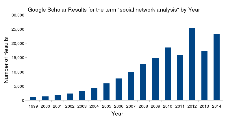
SNA is the study of the network of relationships among a set of things rather than the things themselves. This type of analysis is increasing common in academia across a huge number of fields. Google Scholar gives a fairly clear indication that the term is increasingly common among the academic databases it crawls.

The growth of Social Network Analysis
The growth of Social Network Analysis.

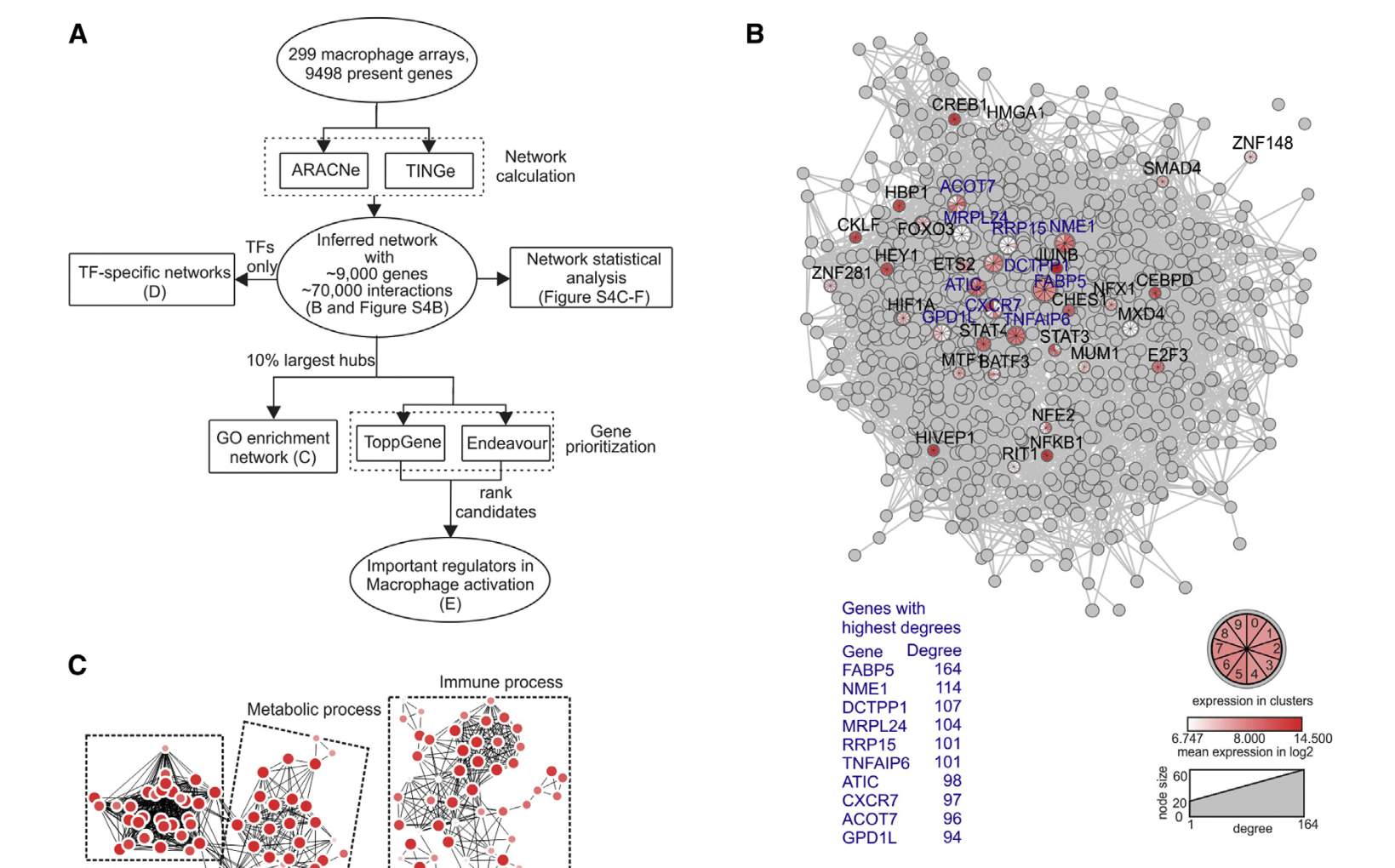
The technique surfaces in many domains, used to identify which actors within a given network are “interesting”. In a biology context “interesting” actors might be the genes that are interacting the most with other genes given a certain stimulus.

 Transcriptome-Based Network Analysis Reveals a Spectrum Model of Human Macrophage Activation Xue, Jia et al.
Transcriptome-Based Network Analysis Reveals a Spectrum Model of Human Macrophage Activation – Xue, Jia et al.

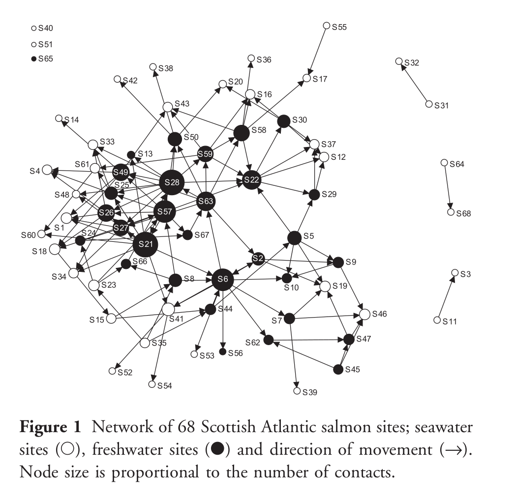
In the context of epidemiology, if the actors are fish farms, the movement of fish between then forms a network which can be analysed. Aquaculture sites that have the highest number of incoming and outgoing connections become “interesting” since the movements mean a high vulnerability to infection and likelihood to spread disease.

Image from the paper Application of network analysis to farmed salmonid movement data from Scotland
Image from the paper Application of network analysis to farmed salmonid
movement data from Scotland

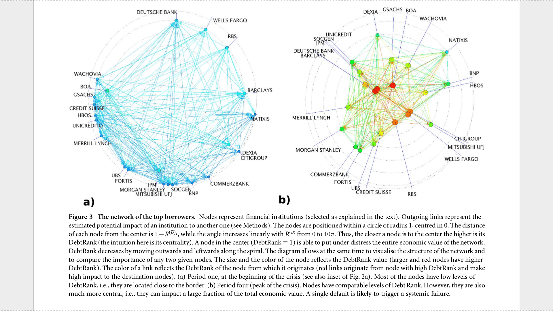
An “interesting” financial institution might be one whose financial ties with other institutions indicate that it’s failure might have a domino effect.

Figure from DebtRank: Too Central to Fail? Financial Networks, the FED and Systemic Risk
Figure from DebtRank: Too Central to Fail? Financial
Networks, the FED and Systemic Risk

While Social Network analysis has been steadily growing, shifts in industry are underway that promise to make this type of analysis more common outside academia.

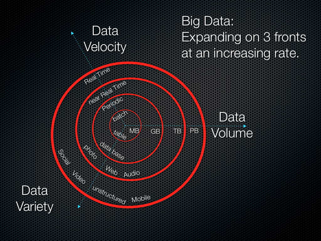
In 2001, with computers spreading everywhere, e-commerce heating up and internet usage around 500 million, Doug Laney, an eagle-eyed analyst for MetaGroup (now Gartner), notices a trend; data is changing. He described how data was increasing along 3 axes: increasing in volume, velocity and variety which eventually became known as “the 3 V’s of Big Data”.

An amazing visualization of the 3 V's from Datasciencecentral.com
An amazing vizualization of the 3 V’s from Datasciencecentral.com

This changing characteristics of data itself has touched off what is often called a “Cambrian explosion” of non-relational databases that offer the speed, flexibility and horizontal scalability needed to accommodate it. These databases and collectively known as NoSQL databases.

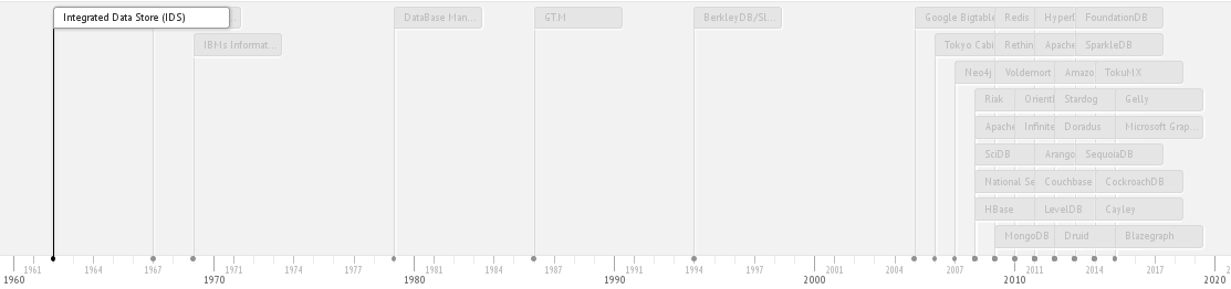
A non-exhaustive but representative timeline of NoSQL databases.
A non-exhaustive but representative timeline of NoSQL databases. From the first database (a graph database) till today. Can you see the explosion? Explore the timeline yourself.

Since the launch of Google’s Bigtable in 2005, More than 28 NoSQL databases have been launched. The majority fall into one of the 3 main sub-categories: key/value store, document store or graph database.

Anywhere a graph database is used is an obvious place to use SNA, but the ability to build a graph atop either key/value stores or document databases means that the majority of NoSQL databases are amenable to being analysed with SNA.

There are also many relational databases struggling to contain and query graphy datasets that developers have dutifully pounded into the shape of a table. As graph databases gain more traction we will likely see some of these converted in their entirety to graphs using tools like R2G wherever developers end up struggling with recursion or an explosion of join tables, or something like routing.

In addition to the steady pressure of the 3 V’s and the growth of SNA as an analytical and even predictive, tool, there are many companies (RunkeeperYahooLinkedIn) whose data model is a graph. Facebook and Netflix both fall into this category and have each released tools, both of which are pitched as alternatives to REST architecture style most web applications are based on, to make building graph backed applications easier.

Circling back to the original question of “why graphs?”, hopefully the answer is clearer. For anyone with an interest in data analysis, paying attention to this space gives access to powerful tools and a growing number of opportunities to apply them. For developers, understanding graphs allows better data modelling and architectural decisions.

Beyond the skills needed to design and tend to these new databases and make sense of their contents, knowledge of graphs will also increasingly be required to make sense of the world around us.

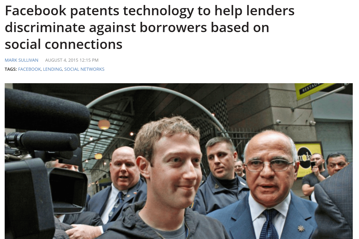
Understanding why you got turned down for a loan will require understanding a graph, why you are/aren’t fat, and eventually who gets insurance and at what price will too.

Facebook patents technology to help lenders discriminate against borrowers based on social connections

Proper security increasingly requires thinking in graphs, as even the most “boring” of us can be a useful stepping stone on the way to compromising someone “interesting”; perhaps a client, an acquaintance, an employer, or a user of something we create.

Graphs will be used to find and eliminate key terrorists, map out criminal networks, and route you to that new vegan restaurant across town.

With talk of storage capacities actually surpassing Moore’s law, SNA growing nearly linearly, NoSQL growing, interest in graphs on the way up, and application development tools finally appearing, the answer to “why now?” is that this is only the beginning. We are all connected, and understanding how is the future.

When to use a graph database

There are a lot of “intro to graph database” tutorials on the internet. While the “how” part of using a graph database has it’s place, I don’t know if enough has been said about “when”.

The answer to “when” depends on the properties of the data you are working with. In broad strokes, you should probably keep a graph database in mind if you are dealing with a significant amount of any of the following:

  • Hierarchical data

  • Connected data

  • Semi-structured data

  • Data with Polymorphic associations

Each of these data types either requires some number of extra tables or columns (or both) to deal with under the relational model. The cost of these extra tables and columns is an increase in complexity.

Terms like “connected data” or “semi-structured data” get used a lot in the NoSQL world but the definitions, where you can find one at all, have a “you’ll know it when you see it” flavour to them. “You’ll know it when you see it” can be distinctly unsatisfying when examples are hard to come by as well. Lets take a look at these one by one and get a sense of they mean generally and how to recognize them in existing relational database backed projects.

Hierarchical Data

Hierarchies show up everywhere. There are geographical hierarchies where a country has many provinces, which have many cities which have many towns. There is also the taxonomic rank, indicating the level of a taxon in the Taxonomic Hierarchy, organizational hierarchies, the North American Industry Classification system… the list goes on and on.

What it looks like in a relational database.

Usually its easy to tell if you are dealing with this type of data. In an existing database schema you may see tables with a parent_id column indicating the use of the Adjacency List pattern or left/right columns indicating the use of the Nested Sets pattern. There are many others as well.

Connected Data

Connected data is roughly synonymous with graph data. When we are talking about graph data we mean bits of data, plus information about how those bits of data are related.

What it looks like in a relational database.

Join tables are the most obvious sign that you are storing graph data. Join tables exist solely to act as the target of two one-to-many relationships, each row representing a relationship between two rows in other tables. Cases where you are storing data in the join table (such as the Rails has_many :through relationship) are even more clear, since the columns of your join table are attributes of an edge.

While one-to-many relationships also technically describe a graph, they probably are not going to make you reconsider the use of a relational database the way large numbers of many-to-many relationships might.

Semi-structured Data

Attempts to define semi-structured data seem to focus on variability; just because one piece of data has a particular set of attributes does not mean that the rest do. You can actually get an example of semi-structured data by mashing together two sets of structured (tabular) data. In this world of APIs and SOA where drawing data from multiple sources is pretty much the new normal, semi-structured data is increasingly common.

What it looks like in a relational database.

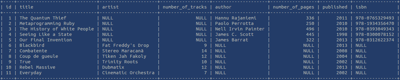
Anywhere you have columns with lots of null values in them. The columns provide the structure, but long stretches of null values suggest that this data does not really fit that structure.

semi_structured_data
An example of semi-structured data: a hypothetical products table combining books (structured data) and music (also structured data).

Polymorphic associations

Having one type data with an association that might be to related to one of two or more things, that’s what known as a polymorphic association. As an example, a photo might be related to a user or a product.

What it looks like in a relational database.

While polymorphic relations can be done in a relational database most commonly they are handled at the framework level, where the framework a foreign key and an additional “type” column to determine the correct table/row. Seeing both an something_id and something_type in the same table gives a hint that a polymorphic relationship is being used. Both Ruby on Rails and Java’s Spring Framework offer this.

So when?

These types of data are known to be an awkward fit for the relational model, in the same way that storing large quantities of perfectly tabular data would be awkward under the graph model. These are ultimately threshold problems, like the famous paradox of the heap.

1000000 grains of sand is a heap of sand

A heap of sand minus one grain is still a heap.

Your first join table or set of polymorphic relations will leave you will a perfectly reasonable database design, but just as “a heap of sand minus one grain” will eventually cross some ill defined threshold and produce something that is no longer a heap of sand, there is some number of join tables or other workarounds for the relational model that will leave you with a database that is significantly more complex than a graph database equivalent would be.

Knowing about the limits of the relational model and doing some hard thinking about how much time you are spending pressed up against those limits is really the only things that can guide your decision making.

Getting started with graph databases

I have a personal project I have been chipping away on for a little while now. I’ve been slowly adding more and more test data to it and as I do its become increasingly clear that while the data itself is neat, the stuff that is actually interesting is actually the relationships between the various entities and not so much the entities themselves. This realization led me to do some reading about graph databases. O’Reilly (as usual) has an interesting book on Graph Databases written by Ian Robinson, Jim Webber, and Emil Eifrem. Its a good intro but given that they hold positions of engineer, chief scientist and CEO at the company that makes the Neo4j graph database, its unsurprisingly focused on Neo4j.

Unfortunately the ‘j’ part of Neo4j refers to Java, which is a whole can of worms that I would rather not open. So I set off to look for a graph database that would not force me onto the JVM, or trap me with open-core licencing (or an $18,000 per year cost for my startup), and ultimately found ArangoDB.

Licenced under Apache 2, ArangoDB (formerly AvacadoDB) is a document database, in the same vein as MongoDB. What’s interesting is that it can also do key/value stuff like Redis and graphs like Neo4j.
Since its written in C++ I don’t have to worry about the JVM. So, lets get started with with it!

Installation is painless on Ubuntu:

wget -qO - http://www.arangodb.org/repositories/arangodb2/xUbuntu_13.10/Release.key | sudo apt-key add -
sudo sh -c "echo 'deb http://www.arangodb.org/repositories/arangodb2/xUbuntu_13.10/ /' > /etc/apt/sources.list.d/arangodb.list"
sudo apt-get update && sudo apt-get install arangodb

Since this is my first contact with graphs, I want a dataset that I can get a feel for working with graphs. Fortunately the company behind ArangoDB (triAGENS) has put some sample data up on github to get people started:

$> git clone https://github.com/triAGENS/ArangoDB-Data.git
Cloning into 'ArangoDB-Data'...
...
$> cd ArangoDB-Data/Graphs/IMDB
$> ./import.sh

That import script imports a bunch of IMDB data into ArangoDB and means that we can start exploring with the arango shell:

$> arangosh

                                       _     
  __ _ _ __ __ _ _ __   __ _  ___  ___| |__  
 / _` | '__/ _` | '_ \ / _` |/ _ \/ __| '_ \ 
| (_| | | | (_| | | | | (_| | (_) \__ \ | | |
 \__,_|_|  \__,_|_| |_|\__, |\___/|___/_| |_|
                       |___/                 

Welcome to arangosh 2.0.2 [linux]. Copyright (c) triAGENS GmbH
Using Google V8 3.16.14 JavaScript engine, READLINE 6.2, ICU 4.8.1.1

Pretty printing values.
Connected to ArangoDB 'tcp://localhost:8529' version: 2.0.2, database: '_system', username: 'root'

use 'help' to see common examples
arangosh [_system]>

Tab completion works super well here to give a sense of what your options are, but the first thing we care about is figuring out what that import did for us. You can see it created two collections (imdb_vertices and imdb_edges) with the db._collections() function:

arangosh [_system]> db._collections()
[ 
  [ArangoCollection 3021163, "_aal" (type document, status loaded)], 
  [ArangoCollection 1317227, "_graphs" (type document, status loaded)], 
  [ArangoCollection 3545451, "_replication" (type document, status loaded)], 
  [ArangoCollection 137579, "_users" (type document, status loaded)], 
  [ArangoCollection 1513835, "_cluster_kickstarter_plans" (type document, status loaded)], 
  [ArangoCollection 940644715, "vertices" (type document, status loaded)], 
  [ArangoCollection 3414379, "_aqlfunctions" (type document, status loaded)], 
  [ArangoCollection 1382763, "_modules" (type document, status loaded)], 
  [ArangoCollection 3610987, "_statistics" (type document, status loaded)], 
  [ArangoCollection 1160255851, "imdb_vertices" (type document, status loaded)], 
  [ArangoCollection 940710251, "edges" (type edge, status loaded)], 
  [ArangoCollection 3479915, "_trx" (type document, status loaded)], 
  [ArangoCollection 266194196843, "imdb_edges" (type edge, status loaded)], 
  [ArangoCollection 1448299, "_routing" (type document, status loaded)] 
]

We can also pick random documents out of the vertices collection with the .any() function to get a sense of whats in there.

 db.imdb_vertices.any()
{ 
  "_id" : "imdb_vertices/40233", 
  "_rev" : "6407199083", 
  "_key" : "40233", 
  "version" : 21, 
  "id" : "65952", 
  "type" : "Person", 
  "birthplace" : "", 
  "biography" : "", 
  "label" : "Jude Poyer", 
  "lastModified" : "1301901667000", 
  "name" : "Jude Poyer" 
}

If you have spent any time on the internet you will of course know that the obvious use for an IMDB graph is calculate Bacon numbers. So lets see if we can find Kevin in here:

arangosh [_system]> db._query('FOR Person IN imdb_vertices FILTER Person.name == "Kevin Bacon" RETURN Person').toArray()
[ 
  { 
    "_id" : "imdb_vertices/759", 
    "_rev" : "1218713963", 
    "_key" : "759", 
    "version" : 146, 
    "id" : "4724", 
    "type" : "Person", 
    "biography" : "", 
    "label" : "Kevin Bacon", 
    "lastModified" : "1299491319000", 
    "name" : "Kevin Bacon", 
    "birthplace" : "Philadelphia", 
    "profileImageUrl" : "http://cf1.imgobject.com/profiles/3e0/4bed49cf017a3c37a30003e0/kevin-bacon-profi...", 
    "birthday" : "-362451600000" 
  } 
]

And let’s see if we can connect him to, say, Kate Winslet. Since we know that Kevin is id imdb_vertices/759 and a little digging shows that Kate’s id is imdb_vertices/1088. We can pass those ids along with the imdb_vertices and imdb_edges collections to the SHORTEST_PATH function ArangoDB supplies for it to make the link between them:

arangosh [_system]> db._query('RETURN SHORTEST_PATH(imdb_vertices, imdb_edges, "imdb_vertices/759", "imdb_vertices/1088", "any", { maxIterations: 100000})').toArray()
[ 
  [ 
    { 
      "vertex" : { 
        "_id" : "imdb_vertices/759", 
        "_rev" : "1218713963", 
        "_key" : "759", 
        "version" : 146, 
        "id" : "4724", 
        "type" : "Person", 
        "biography" : "", 
        "label" : "Kevin Bacon", 
        "lastModified" : "1299491319000", 
        "name" : "Kevin Bacon", 
        "birthplace" : "Philadelphia", 
        "profileImageUrl" : "http://cf1.imgobject.com/profiles/3e0/4bed49cf017a3c37a30003e0/kevin-bacon-profi...", 
        "birthday" : "-362451600000" 
      } 
    }, 
    { 
      "vertex" : { 
        "_id" : "imdb_vertices/35451", 
        "_rev" : "5779626347", 
        "_key" : "35451", 
        "runtime" : 87, 
        "version" : 186, 
        "id" : "9692", 
        "genre" : "Drama", 
        "language" : "en", 
        "type" : "Movie", 
        "homepage" : "", 
        "tagline" : "", 
        "title" : "The Woodsman", 
        "label" : "The Woodsman", 
        "description" : "A pedophile returns to his hometown after 12 years in prison and attempts to sta...", 
        "imdbId" : "tt0361127", 
        "lastModified" : "1301903901000", 
        "imageUrl" : "http://cf1.imgobject.com/posters/3c1/4bc9281e017a3c57fe0103c1/the-woodsman-mid.j...", 
        "studio" : "Dash Films", 
        "releaseDate" : "1103842800000", 
        "released" : "2000-2010" 
      } 
    }, 
    { 
      "vertex" : { 
        "_id" : "imdb_vertices/1179", 
        "_rev" : "1274747243", 
        "_key" : "1179", 
        "version" : 90, 
        "id" : "335", 
        "type" : "Person", 
        "biography" : "", 
        "label" : "Michael Shannon", 
        "lastModified" : "1299902807000", 
        "name" : "Michael Shannon", 
        "profileImageUrl" : "http://cf1.imgobject.com/profiles/01c/4c2a3dc87b9aa15e9900001c/michael-shannon-p..." 
      } 
    }, 
    { 
      "vertex" : { 
        "_id" : "imdb_vertices/21077", 
        "_rev" : "3892517227", 
        "_key" : "21077", 
        "runtime" : 119, 
        "version" : 339, 
        "id" : "4148", 
        "genre" : "Drama", 
        "language" : "en", 
        "type" : "Movie", 
        "homepage" : "", 
        "tagline" : "", 
        "title" : "Revolutionary Road", 
        "label" : "Revolutionary Road", 
        "description" : "A young couple living in a Connecticut suburb during the mid-1950s struggle to c...", 
        "imdbId" : "tt0959337", 
        "trailer" : "http://www.youtube.com/watch?v=af01__Kvvr8", 
        "lastModified" : "1301907499000", 
        "imageUrl" : "http://cf1.imgobject.com/posters/627/4d4f8e275e73d617b7003627/revolutionary-road...", 
        "studio" : "BBC Films", 
        "releaseDate" : "1229641200000", 
        "released" : "2000-2010" 
      } 
    }, 
    { 
      "vertex" : { 
        "_id" : "imdb_vertices/1088", 
        "_rev" : "1262754155", 
        "_key" : "1088", 
        "version" : 102, 
        "id" : "204", 
        "type" : "Person", 
        "label" : "Kate Winslet", 
        "lastModified" : "1299746700000", 
        "name" : "Kate Winslet", 
        "birthplace" : "Reading, UK", 
        "profileImageUrl" : "http://cf1.imgobject.com/profiles/59f/4c022d0e017a3c702d00159f/kate-winslet-prof...", 
        "biography" : "<meta charset=\"utf-8\"><span style=\"font-family: sans-serif; font-size: 18px; lin...", 
        "birthday" : "181695600000" 
      } 
    } 
  ] 
]

So what we can see here is that it takes two hops (from Kevin to Michael Shannon via “The Woodsman“, and from Michael to Kate via “Revolutionary Road“), to connect Kevin Bacon to Kate Winslet, giving her a Bacon number of 2.

For the moment that is as far as I have gotten but I am pretty excited to explore the possiblities here. The more I think about graphs as a data model the more they seem to be a good fit for a lot of problems that I would normally be forcing into tables. Given that I can also just do straight document storage and the fact that they have a Object Document Mapper that works with Rails, I can tell you that ArangoDB and I will be spending a lot of time together.